A 120,000-year long climate record from a NW-Greenland deep ice core at ultra-high resolution
We report high resolution measurements of the stable isotope ratios of ancient ice (δ 18 O, δD) from the North Greenland Eemian deep ice core (NEEM, 77.45° N, 51.06° E). The record covers the period 8–130 ky b2k (y before 2000) with a temporal resolution of ≈0.5 and 7 y at the top and the bottom of the core respectively and contains important climate events such as the 8.2 ky event, the last glacial termination and a series of glacial stadials and interstadials. At its bottom part the record contains ice from the Eemian interglacial. Isotope ratios are calibrated on the SMOW/SLAP scale and reported on the GICC05 (Greenland Ice Core Chronology 2005) and AICC2012 (Antarctic Ice Core Chronology 2012) time scales interpolated accordingly. We also provide estimates for measurement precision and accuracy for both δ 18 O and δD.
isotope analysis • water ice core
cavity ring-down spectroscopy
Sample Characteristic - Location
Greenland Ice Sheet
Machine-accessible metadata file describing the reported data: https://doi.org/10.6084/m9.figshare.14216441
Two-million-year-old snapshots of atmospheric gases from Antarctic ice
Article 30 October 2019

Abrupt Common Era hydroclimate shifts drive west Greenland ice cap change
Article 09 September 2021
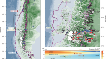
Near-synchronous Northern Hemisphere and Patagonian Ice Sheet variation over the last glacial cycle
Article 08 May 2024
Background & Summary
Stable water isotope analysis has traditionally been performed with Isotope Ratio Mass Spectrometry (IRMS) utilising an array of different implementations, each one presenting advantages and disadvantages with respect to precision, accuracy, sample consumption and throughput, as well as ease of use and labour intensity 15,16,17,18,19 . With the advent of fast electronics and room-temperature, turn-key, solid state laser sources, there emerged various optical spectroscopic techniques, typically in the near Infra-Red spectral region that allowed for quasi-simultaneous analysis of the three isotope ratios 2 H/ 1 H, 17 O/ 16 O and 18 O/ 16 O on the same water sample 20,21 . Commercial instruments using Cavity Enhanced Spectroscopic techniques allowed for routine simultaneous measurements of δ 18 O and δD using a greatly reduced amount of sample and with precision and accuracy comparable, if not better than that of IRMS 22,23 . The new techniques offered the possibility for in-situ measurements of the isotopic composition of vapour 24,25,26 while in combination with continuous melter systems, and micro-volume flash vaporisers, they yielded ice core data sets of unprecedented resolution 23,27,28,29,30,31 .
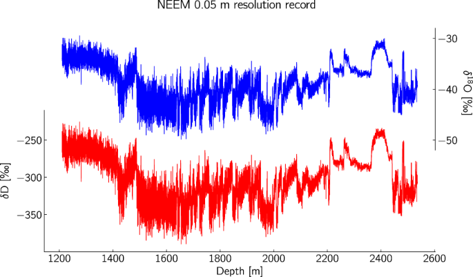
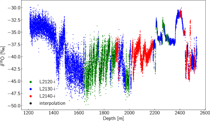
Here, we present a high-resolution (0.05 m) water isotope (δ 18 O and δD) record 32 from the Greenland NEEM ice core, drilled from 2007 to 2012 at 77.45°N–51.06°W. The record covers the segment of the ice core below 1210.5 m - a depth that corresponds to an age of 8000 y b2k (y before 2000 AD)- and extends to a final depth of 2536.5 m. The oldest age of the record is 129,258 y b2k at the depth of 2432.15 m. We report ages on the GICC05 (ages 8–121.446 ky b2k) and the AICC2012 (ages 60–129.258 ky b2k) time scales interpolated accordingly. Beyond that point and for the deepest 104 m, an age scale cannot be reconstructed as the record is too disturbed due to ice folds 33 .
Isotopic analysis has been performed using Laser Spectroscopy and in particular three different versions of the Cavity Ring Down Spectrometers (CRDS) from Picarro Inc. (L2120-i, L2130-i, L2140-i). All measurements are reported on the international VSMOW-SLAP (VSMOW and SLAP refer to the International Atomic Energy reference water materials and stand for Vienna Mean Ocean Water and Standard Light Antarctic Precipitation) isotope scale after careful calibration using a triplet of local standards calibrated against the primary International Atomic Energy Agency reference materials. We describe the methodology of the measurement including information on instrument calibration procedures and an accuracy and precision assessment.
The dataset will be useful for future studies of past climate variability on long (millennial) and short (decadal to annual) time scales. Studies focusing on the spectral properties of the isotopic signal will also benefit from the high resolution apparent in the record. The record includes significant past-climate events such as the 8.2 ky climatic transition, the last Glacial Termination, as well as the series of Glacial Stadial-Interstadials of the last 120 ky (GI-1, GS-1 to GI-25c, GS-26)0 34 .
Methods
Discrete Ice Core Sampling
The sampling of the ice core for water isotope analysis was performed in the field during the field seasons 2009–2012. A wedge with a cross section of approximately 10 cm 2 (roughly 12% of the cross section of the ice core) was cut using a band saw with a resolution of 0.025 m for the top 601.7 m and 0.05 m for the interval 601.75–2536.5 (Fig. 1). The dataset presented here, has a resolution of 0.05 m. The ice samples were stored and transported to Copenhagen, Denmark frozen in plastic bags for further preparation and isotopic analysis.
Subsequently, and after arrival to the Stable Isotope Lab at the Niels Bohr Institute, the samples were melted at room temperature in air-tight containers and transferred to 10 ml PE-LD narrow mouth bottles (VITLAB-138093). From that point, the samples were stored frozen until the time of isotopic analysis using CRDS. Prior to analysis, 200 μl of sample were transferred from the PE-LD bottles to 2 ml short thread glass vials with integrated 300 μl micro-inserts (La-Pha-Pack 11092357) sealed with triple layer Teflon/Silicon/Teflon caps (La-Pha-Pack 09150480).
Stable isotope analysis
Cavity ring down spectroscopy
Isotope analysis is performed with Cavity Ring Down Spectroscopy (CRDS) in the near Infra-Red region. For this study, we have used three different models of the Picarro L21XX-i analyser namely the L2120-i, L2130-i and L2140-i. The record contains a total of 26,519 data points acquired with the three instruments. The exact number of data points per instrument is given in Table 1.
Tray configuration - PAL Autosampler jobs sequence
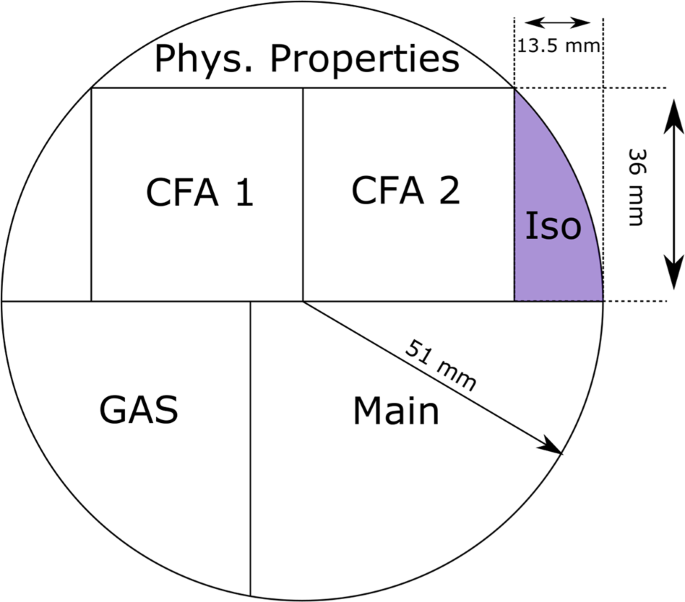
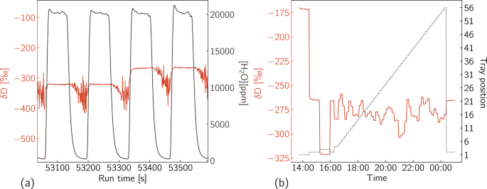
In Table 3 we describe the sequence of the PAL autosampler jobs and the tray configuration. The measurement run begins with the VSMOW-SLAP calibration block (Vials #1 and #3) followed by the unknown (with the term “unknown” here we refer to the ice core samples whose isotopic composition is to be measured) samples run sequentially with increasing depth (Vials #4–56). A measurement of every local water standard consists of 20 injections of which the first 12 are discarded, in order to account for memory effects caused by the large isotopic step between the standards. The measurement of the unknowns is based on a block of four injections of which the first one is discarded. Three blocks containing a “check” standard that is treated as an unknown (Vial #2) are introduced in the middle and at the end of the VSMOW-SLAP calibration as well as at the end of the run after all unknowns have been measured. The “check” standard provides a measure of the obtained accuracy as well as the long term stability of the run. In total, 300 injections are performed, resulting to a total run duration of approximately 11 hours and 40 minutes. A complete run is illustrated in Fig. 2.
Technical Validation
Measurement precision and accuracy
The measurement precision of every run, is estimated from the calculation of the standard deviation of the valid injections of the “check” standard blocks (Vial #2). Measurement precision is given for δ 18 O and δD in columns 8 and 9 of the data set. Similarly, the difference between the assigned and the post-calibration value of the “check” standard is used as a measure of the accuracy of the run. This metric is given in columns 10 and 11 for δ 18 O and δD respectively.
In Fig. 5 we plot the two metrics as a function of depth categorised by the instrument type and in Fig. 6 we bin the data points in histograms. From these two figures it is apparent that the performance of the L2130-i and L2140-i versions of the CRDS spectrometer is superior to that of the L2120-i version. The difference in performance concerns both the precision and the accuracy of the measurement and it appears to be more profound for the δ 18 O measurement. This behaviour is explained by the more accurate spectroscopic corrections, as well as the more precise control of the optical cavity’s temperature and pressure of the newer L2130-i and L2140-i models. The statistics of the distributions for the two metrics are outlined in Table 6. Based on the data of Table 6 we can commend that the obtained accuracy as expressed by the “check” standard offset, is well within the 2σ (95%) interval as defined by the precision of the “check” standard measurement for all the runs of the record.
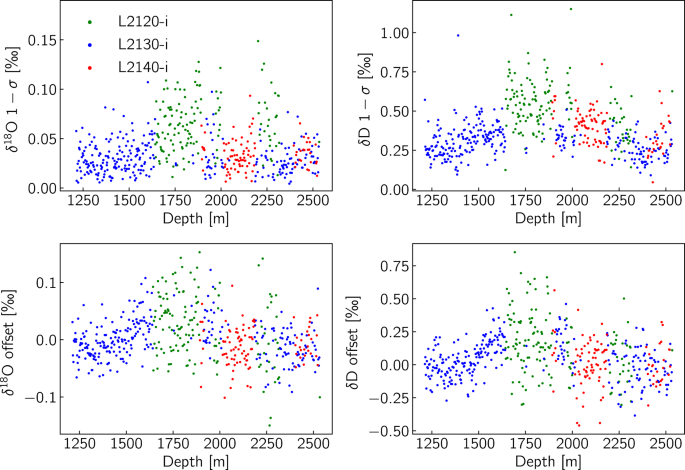
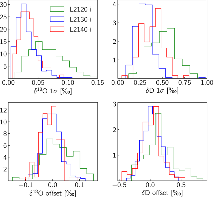
Table 6 Statistics of the “check” standard quality-control metrics as presented in Fig. 6 for the three instrument types.
Code availability
The Python code used for the transfer, organising of the data, estimation of the precision and accuracy metrics as well as the plots included in this manuscript can be found in https://github.com/vgkinis/neem_isotope_data_descriptor_code. In the repository, we also provide auxiliary code with basic routines for post-processing of the PANGAEA data file.
References
- Dansgaard, W. Stable isotopes in precipitation. Tellus16, 436–468, https://doi.org/10.3402/tellusa.v16i4.8993 (1964). ArticleADSGoogle Scholar
- Ciais, P. & Jouzel, J. Deuterium and oxygen-18 in precipitation - isotopic model, including mixed cloud processes. J. Geophys. Res.-Atmospheres99, 16793–16803, https://doi.org/10.1029/94JD00412 (1994). ArticleADSCASGoogle Scholar
- Jouzel, J. et al. Validity of the temperature reconstruction from water isotopes in ice cores. J. Geophys. Res.-Oceans102, 26471–26487, https://doi.org/10.1029/97JC01283 (1997). ArticleADSCASGoogle Scholar
- Jouzel, J. A brief history of ice core science over the last 50 yr. Clim. Past9, 2525–2547, https://doi.org/10.5194/cp-9-2525-2013 (2013). ArticleGoogle Scholar
- NGRIP members. High-resolution record of Northern Hemisphere climate extending into the last interglacial period. Nature431, 147–151, https://doi.org/10.1038/nature02805 (2004). ArticleCASGoogle Scholar
- EPICA Community Members. Eight glacial cycles from an Antarctic ice core. Nature429, 623–628, https://doi.org/10.1038/nature02599 (2004). ArticleCASGoogle Scholar
- Steffensen, J. P. et al. High-resolution Greenland ice core data show abrupt climate change happens in few years. Science321, 680–684, https://doi.org/10.1126/science.1157707 (2008). ArticleADSCASPubMedGoogle Scholar
- Vinther, B. M. et al. A synchronized dating of three Greenland ice cores throughout the Holocene. J. Geophys. Res.-Atmospheres111, D13102, https://doi.org/10.1029/2005JD006921 (2006). ArticleADSGoogle Scholar
- Rasmussen, S. O. et al. A new Greenland ice core chronology for the last glacial termination. J. Geophys. Res.111, D06102, https://doi.org/10.1029/2005JD006079 (2006). ArticleADSCASGoogle Scholar
- Masson-Delmotte, V. et al. GRIP Deuterium excess reveals rapid and orbital-scale changes in Greenland moisture origin. Science309, 118–121, https://doi.org/10.1126/science.1108575 (2005). ArticleADSCASPubMedGoogle Scholar
- Gkinis, V., Simonsen, S. B., Buchardt, S. L., White, J. W. C. & Vinther, B. M. Water isotope diffusion rates from the NorthGRIP ice core for the last 16,000 years - Glaciological and paleoclimatic implications. Earth and Planetary Science Letters405, 132–141, https://doi.org/10.1016/j.epsl.2014.08.022 (2014). ArticleADSCASGoogle Scholar
- Buizert, C. et al. Greenland temperature response to climate forcing during the last deglaciation. Science (New York, N.Y.)345, 1177–1180, https://doi.org/10.1126/science.1254961 (2014). ArticleADSCASGoogle Scholar
- Jones, T. R. et al. Southern Hemisphere climate variability forced by Northern Hemisphere ice-sheet topography. Nature554, 351–355, https://doi.org/10.1038/nature24669 (2018). ArticleADSCASPubMedGoogle Scholar
- Holme, C., Gkinis, V. & Vinther, B. M. Molecular diffusion of stable water isotopes in polar firn as a proxy for past temperatures. Geochim. Cosmochim. Acta225, 128–145, https://doi.org/10.1016/j.gca.2018.01.015 (2018). ArticleADSCASGoogle Scholar
- Bigeleisen, J., Perlman, M. L. & Prosser, H. C. Conversion of Hydrogenic Materials to Hydrogen for Isotopic Analysis. Analytical Chemistry24, 1356–1357, https://doi.org/10.1021/ac60068a025 (1952). ArticleCASGoogle Scholar
- Epstein, T. & Mayeda, S. Variations of 18 O content of waters from natural sources. Geochim. Cosmochim. Acta4, 213–224, https://doi.org/10.1016/0016-7037(53)90051-9 (1953). ArticleADSCASGoogle Scholar
- Vaughn, B. H. et al. An automated system for hydrogen isotope analysis of water. Chemical Geology152, 309–319, https://doi.org/10.1016/S0009-2541(98)00117-X (1998). ArticleADSCASGoogle Scholar
- Begley, I. S. & Scrimgeour, C. M. High-precision δ 2 H and δ 18 O measurement for water and volatile organic compounds by Continuous-Flow Pyrolysis Isotope Ratio Mass Spectrometry. Analytical Chemistry69, 1530–1535, https://doi.org/10.1021/ac960935r (1997). ArticleCASGoogle Scholar
- Gehre, M., Geilmann, H., Richter, J., Werner, R. A. & Brand, W. A. Continuous flow 2 H/ 2 H and δ 18 O analysis of water samples with dual inlet precision. Rapid Communications In Mass Spectrometry18, 2650–2660, https://doi.org/10.1002/rcm.1672 (2004). ArticleADSCASPubMedGoogle Scholar
- Kerstel, E. R. T., van Trigt, R., Dam, N., Reuss, J. & Meijer, H. A. J. Simultaneous determination of the 2 H/ 1 H, 17 O/ 16 O and 18 O/ 16 O isotope abundance ratios in water by means of laser spectrometry. Analytical Chemistry71, 5297–5303, https://doi.org/10.1021/ac990621e (1999). ArticleCASPubMedGoogle Scholar
- Van Trigt, R., Meijer, H. A. J., Sveinbjörnsdóttir, A. E., Johnsen, S. J. & Kerstel, E. R. T. Measuring stable isotopes of Hydrogen and Oxygen in ice by means of laser spectrometry: the Bølling transition in the Dye-3 (south Greenland) ice core. Ann. Glaciol.35, 125–130, https://doi.org/10.3189/172756402781816906 (2002). ArticleADSGoogle Scholar
- Crosson, E. R. A cavity ring-down analyzer for measuring atmospheric levels of methane, carbon dioxide, and water vapor. Applied Physics B-Lasers And Optics92, 403–408, https://doi.org/10.1063/1.1139895 (2008). ArticleADSCASGoogle Scholar
- Gkinis, V., Popp, T. J., Johnsen, S. J. & Blunier, T. A continuous stream flash evaporator for the calibration of an IR cavity ring-down spectrometer for the isotopic analysis of water. Isotopes In Environmental and Health Studies46, 463–475, https://doi.org/10.1080/10256016.2010.538052 (2010). ArticleCASPubMedGoogle Scholar
- Aemisegger, F. et al. Measuring variations of δ 18 O and δ 2 H in atmospheric water vapour using two commercial laser-based spectrometers: an instrument characterisation study. Atmos. Meas. Tech.5, 1491–1511, https://doi.org/10.5194/amt-5-1491-2012 (2012). ArticleCASGoogle Scholar
- Steen-Larsen, H. C. et al. Continuous monitoring of summer surface water vapor isotopic composition above the Greenland Ice Sheet. Atmos. Chem. Phys.13, 4815–4828, https://doi.org/10.5194/acp-13-4815-2013 (2013). ArticleADSCASGoogle Scholar
- Benetti, M. et al. Stable isotopes in the atmospheric marine boundary layer water vapour over the Atlantic Ocean, 2012–2015. Sci. Data 160128, https://doi.org/10.1038/sdata.2016.128 (2017).
- Gkinis, V. et al. Water isotopic ratios from a continuously melted ice core sample. Atmos. Meas. Tech.4, 2531–2542, https://doi.org/10.5194/amt-4-2531-2011 (2011). ArticleCASGoogle Scholar
- Maselli, O. J., Fritzsche, D., Layman, L., McConnell, J. R. & Meyer, H. Comparison of water isotope-ratio determinations using two cavity ring-down instruments and classical mass spectrometry in continuous ice-core analysis. Isotopes Environ. Health Stud. 387–398, https://doi.org/10.1080/10256016.2013.781598 (2013).
- Emanuelsson, B. D., Baisden, W. T., Bertler, N. A. N., Keller, E. D. & Gkinis, V. High-resolution continuous-flow analysis setup for water isotopic measurement from ice cores using laser spectroscopy. Atmos. Meas. Tech.8, 2869–2883, https://doi.org/10.5194/amt-8-2869-2015 (2015). ArticleCASGoogle Scholar
- Jones, T. R. et al. Improved methodologies for continuous-flow analysis of stable water isotopes in ice cores. Atmos. Meas. Tech.10, 617–632, https://doi.org/10.5194/amt-10-617-2017 (2017). ArticleADSCASGoogle Scholar
- Jones, T. R. et al. Water isotope diffusion in the WAIS Divide ice core during the Holocene and last glacial. J. Geophys. Res. Earth Surf.122, 290–309, https://doi.org/10.1002/2016JF003938 (2017). ArticleADSCASGoogle Scholar
- Gkinis, V. et al. NEEM ice core High Resolution (0.05 m) Water Isotope Ratios (18 O/16 O, 2H/1H) covering 8-129 ky b2k, https://doi.org/10.1594/PANGAEA.925552 (2020).
- NEEM Community Members. Eemian interglacial reconstructed from a Greenland folded ice core. Nature493, 489–494, https://doi.org/10.1038/nature11789 (2013). ArticleADSCASGoogle Scholar
- Rasmussen, S. O. et al. A stratigraphic framework for abrupt climatic changes during the Last Glacial period based on three synchronized Greenland ice-core records: refining and extending the INTIMATE event stratigraphy. Quat. Sci. Rev.106, 14–28, https://doi.org/10.1016/j.quascirev.2014.09.007 (2014). ArticleADSGoogle Scholar
- Svensson, A. et al. A 60 000 year Greenland stratigraphic ice core chronology. Clim. Past4, 47–57, https://doi.org/10.5194/cp-4-47-2008 (2008). ArticleGoogle Scholar
- Wolff, E. W., Chappellaz, J., Blunier, T., Rasmussen, S. O. & Svensson, A. Millennial-scale variability during the last glacial: The ice core record. Quat. Sci. Rev.29, 2828–2838, https://doi.org/10.1016/j.quascirev.2009.10.013 (2010). ArticleADSGoogle Scholar
- Bazin, L. et al. An optimized multi-proxy, multi-site Antarctic ice and gas orbital chronology (AICC2012): 120-800 ka. Clim. Past9, 1715–1731, https://doi.org/10.5194/cp-9-1715-2013 (2013). ArticleGoogle Scholar
- Veres, D. et al. The Antarctic ice core chronology (AICC2012): an optimized multi-parameter and multi-site dating approach for the last 120 thousand years. Clim. Past9, 1733–1748, https://doi.org/10.5194/cp-9-1733-2013 (2013). ArticleGoogle Scholar
- Rasmussen, S. O. et al. A first chronology for the North Greenland Eemian Ice Drilling (NEEM) ice core. Clim. Past9, 2713–2730, https://doi.org/10.5194/cp-9-2713-2013 (2013). ArticleGoogle Scholar
- Govin, A. et al. Sequence of events from the onset to the demise of the Last Interglacial: Evaluating strengths and limitations of chronologies used in climatic archives. Quat. Sci. Rev.129, 1–36, https://doi.org/10.1016/j.quascirev.2015.09.018 (2015). ArticleADSGoogle Scholar
- Andersen, K. K. et al. The Greenland Ice Core Chronology 2005, 15-42 ka. Part 1: constructing the time scale. Quat. Sci. Rev.25, 3246–3257, https://doi.org/10.1016/j.quascirev.2006.08.002 (2006). ArticleADSGoogle Scholar
- Ruth, U. et al. “EDML1”: a chronology for the EPICA deep ice core from Dronning Maud Land, Antarctica, over the last 150 000 years. Clim. Past3, 475–484, https://doi.org/10.5194/cp-3-475-2007 (2007). ArticleGoogle Scholar
Acknowledgements
We are grateful to the drilling engineers, operators and field assistants that made the retrieval, processing and distribution of the NEEM ice core possible. We would like to acknowledge financial support from the European Research Council under European Union’s Seventh Framework Programme for research and innovation (FP7-ENVIRONMENT grant agreement ID: 243908; FP7-IDEAS-ERC grant agreement ID: 246815, 610055; Marie Sklodowska-Curie grant agreement ID: 600207), the Villum Foundation (Grant 00022995, 000280161, 16572), the US National Science Foundation (Award 0806387), the French National Research Agency (grants ANR-07-VULN-0009, ANR-19-MPGA-0001). NEEM is directed and organised by the Centre of Ice and Climate at the Niels Bohr Institute, funded by the Danish National Research Foundation and US NSF, Office of Polar Programs. It is supported by funding agencies and institutions in Belgium (FNRS-CFB and FWO), Canada (NRCan/GSC), China (CAS), Denmark (FIST), France (IPEV, CNRS/INSU, CEA and ANR), Germany (AWI), Iceland (RannIs), Japan (NIPR), South Korea (KOPRI), the Netherlands (NWO/ALW), Sweden (VR), Switzerland (SNF), the United Kingdom (NERC) and the US (US NSF, Office of Polar Programs) and the EU Seventh Framework Programmes Past4Future and WaterundertheIce.
Author information
Authors and Affiliations
- Physics of Ice Climate and Earth, Niels Bohr Institute, University of Copenhagen, Tagensvej 16, 2200, Copenhagen, Denmark Vasileios Gkinis, Bo M. Vinther, Trevor J. Popp, Thea Quistgaard, Anne-Katrine Faber, Christian T. Holme, Camilla-Marie Jensen, Mika Lanzky, Anine-Maria Lütt, Vasileios Mandrakis, Niels-Ole Ørum, Anna-Sofie Pedersen, Nikol Vaxevani, Yongbiao Weng, Emilie Capron, Dorthe Dahl-Jensen, Sune O. Rasmussen, Hans Christian Steen-Larsen, Jørgen-Peder Steffensen & Anders Svensson
- Geophysical Institute and Bjerknes Centre for Climate Research, University of Bergen, Allégaten 70, 5007, Bergen, Norway Anne-Katrine Faber, Yongbiao Weng & Hans Christian Steen-Larsen
- Climate and Environmental Physics, Physics Institute, Sidlerdtrasse 5, 3012, Bern, Switzerland Camilla-Marie Jensen & Vasileios Mandrakis
- Department of Geosciences, University of Oslo, Sem Sæ lands Vei 1, 0371, Oslo, Norway Mika Lanzky
- Institut des Géosciences de l’Environnement, Université Grenoble Alpes, CNRS, IRD, G-INP, 38000, Grenoble, France Emilie Capron
- Centre for Earth Observation Science, 535 Wallace Building, University of Manitoba, Winnipeg, MB, R3T 2N2, Canada Dorthe Dahl-Jensen
- Alfred-Wegener-Institut Helmholtz-Zentrum für Polar- und Meeresforschung, Am Handelshafen 12, 27570, Bremerhaven, Germany Maria Hörhold & Hans Oerter
- Institute of Arctic and Alpine Research, University of Colorado, Boulder, Colorado, 80309-0450, USA Tyler R. Jones, Bruce Vaughn & James W. C. White
- Laboratoire des Sciences du Climat et de l’Environnement (LSCE), Institut Pierre Simon Laplace (CEA-CNRS-UVSQ UMR 8212), Université Paris Saclay, Gif-sur-Yvette, France Jean Jouzel, Amaëlle Landais & Valérie Masson-Delmotte
- Institute of Earth Sciences, University of Iceland, Sturlugata 7, Reykjavik, Iceland Árný-Erla Sveinbjörnsdóttir
- Vasileios Gkinis
